- AwesomeHive Team
- 0 Comments
- 1582 Views
Although Python or R programming language has a relatively easy learning curve, web developers are just happy to do everything within their comfort zone of JavaScript. Considering the trend that Node.js has started, of applying JavaScript to every field. Python became popular because of the abundance of packages available, but the JS community is not far behind. In this article, we will build a simple classifier in a beginner friendly process.
What you will build
You will make a webpage that uses TensorFlow.js to train a model in the browser. Given “AvgAreaNumberofRooms” for a house, the model will learn to predict “price” of the house.
To do this you will:
- Load the data and prepare it for training.
- Define the architecture of the model.
- Train the model and monitor its performance as it trains.
- Evaluate the trained model by making some predictions.
Step 1: Let us start with the basics.
Create an HTML page and include the JavaScript. Copy the following code into an HTML file called
index.html
<!DOCTYPE html>
<html>
<head>
  <title>TensorFlow.js Tutorial</title>  <!-- Import TensorFlow.js -->
  <script src="https://cdn.jsdelivr.net/npm/@tensorflow/[email protected]/dist/tf.min.js"></script>
  <!-- Import tfjs-vis -->
  <script src="https://cdn.jsdelivr.net/npm/@tensorflow/[email protected]/dist/tfjs-vis.umd.min.js"></script>  <!-- Import the main script file -->
  <script src="script.js"></script></head><body>
</body>
</html>
Create the JavaScript file for the code
In the same folder as the HTML file above, create a file called script.js and put the following code in it.
console.log('Hello TensorFlow');
Test it out
Now that you’ve got the HTML and JavaScript files created, test them out. Open up the index.html file in your browser and open up the devtools console.
If everything is working, there should be two global variables created and available in the devtools console.:
tfis a reference to the TensorFlow.js librarytfvisis a reference to the tfjs-vis library
You should see a message that says Hello TensorFlow. “If so, you are ready to move on to the next step.
Step 2: Load the data, format the data and visualize the input data.
We will load the “house” data-set, which can be found here. It contains many different features for a given house. For this tutorial, we only want data about average area number of rooms and the price of each house.
Add the following code to your script.js file.
async function getData() {
  const houseDataReq = await fetch('https://raw.githubusercontent.com/meetnandu05/ml1/master/house.json');
  const houseData = await houseDataReq.json();
  const cleaned = houseData.map(house => ({
    price: house.Price,
    rooms: house.AvgAreaNumberofRooms,
  }))
  .filter(house => (house.price != null && house.rooms != null));

  return cleaned;
}
This will also remove any entries that do not have either price or number of rooms defined. Let’s also plot this data in a scatterplot to see what it looks like.
Add the following code to the bottom of your script.js file.
async function run() {
  // Load and plot the original input data that we are going to train on.
  const data = await getData();
  const values = data.map(d => ({
    x: d.rooms,
    y: d.price,
  }));  tfvis.render.scatterplot(
    {name: 'No.of rooms v Price'},
    {values},
    {
      xLabel: 'No. of rooms',
      yLabel: 'Price',
      height: 300
    }
  );  // More code will be added below
}document.addEventListener('DOMContentLoaded', run);
When you refresh the page. You should see a panel on the left-hand side of the page with a scatterplot of the data. It should look something like this.
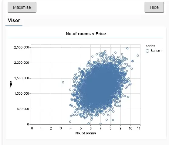
Generally, when working with data it is a good idea to find ways to take a look at your data and clean it if necessary. Visualizing the data can give us a sense of whether there is any structure to the data that the model can learn.
We can see from the plot above that there is a positive correlation between no. of rooms and price, i.e. as no. of rooms increases, prices of houses generally increase.
Step 3: Build the model to be trained.
Here, we will write the code to build our machine learning model. The model will be trained based on this code and hence this is an important step. Machine Learning models take inputs and then produce outputs. In the case of Tensorflow.js, we have to build neural networks.
Add the following function to your script.js file to define the model.
function createModel() {
  // Create a sequential model
  const model = tf.sequential();

  // Add a single hidden layer
  model.add(tf.layers.dense({inputShape: [1], units: 1, useBias: true}));

  // Add an output layer
  model.add(tf.layers.dense({units: 1, useBias: true}));  return model;
}
This is one of the simplest models we can define in tensorflow.js, let us break-down each line a bit.
Instantiate the model
const model = tf.sequential();
This instantiates a tf.Model object. This model is sequential because its inputs flow straight down to its output. Other kinds of models can have branches, or even multiple inputs and outputs, but in many cases your models will be sequential.
Add layers
model.add(tf.layers.dense({inputShape: [1], units: 1, useBias: true}));

This adds a hidden layer to our network. As this is the first layer of the network, we need to define our inputShape. The inputShape is [1] because we have 1number as our input (the number of rooms of a given house).

units sets how big the weight matrix will be in the layer. By setting it to 1 here we are saying there will be 1 weight for each of the input features of the data.

model.add(tf.layers.dense({units: 1}));

The code above creates our output layer. We set units to 1 because we want to output 1 number.
Create an instance

Add the following code to the run function we defined earlier.

// Create the model
const model = createModel();
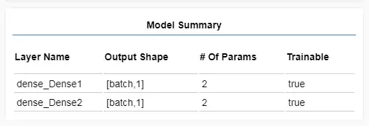
tfvis.show.modelSummary({name: 'Model Summary'}, model);

This will create an instance of the model and show a summary of the layers on the webpage.
Step 4: Prepare the data for training
To get the performance benefits of TensorFlow.js that make training machine learning models practical, we need to convert our data to tensors.
Add the following code to your script.js file
function convertToTensor(data) {

  return tf.tidy(() => {
    // Step 1. Shuffle the data
    tf.util.shuffle(data);    // Step 2. Convert data to Tensor
    const inputs = data.map(d => d.rooms)
    const labels = data.map(d => d.price);    const inputTensor = tf.tensor2d(inputs, [inputs.length, 1]);
    const labelTensor = tf.tensor2d(labels, [labels.length, 1]);    //Step 3. Normalize the data to the range 0 - 1 using min-max scaling
    const inputMax = inputTensor.max();
    const inputMin = inputTensor.min();
    const labelMax = labelTensor.max();
    const labelMin = labelTensor.min();    const normalizedInputs = inputTensor.sub(inputMin).div(inputMax.sub(inputMin));
    const normalizedLabels = labelTensor.sub(labelMin).div(labelMax.sub(labelMin));    return {
      inputs: normalizedInputs,
      labels: normalizedLabels,
      // Return the min/max bounds so we can use them later.
      inputMax,
      inputMin,
      labelMax,
      labelMin,
    }
  });
}
Let’s break down what’s going on here.
Shuffle the data
// Step 1. Shuffle the data
tf.util.shuffle(data);
During training the model, the dataset is divided into smaller sets, each set known as a batch. These batches are then fed to the model for training. Shuffling the data is important because the model should not get the same data over and over again. If the model gets the same data over and over again, the model will not be able to generalize the data and give outputs specified to the inputs it received during training. Shuffling will help by having a variety of data in each batch.
Convert to tensors
// Step 2. Convert data to Tensor
const inputs = data.map(d => d.rooms)
const labels = data.map(d => d.price);const inputTensor = tf.tensor2d(inputs, [inputs.length, 1]);
const labelTensor = tf.tensor2d(labels, [labels.length, 1]);
Here we make two arrays, one for our input examples (the no. of rooms entries), and another for the true output values (which are known as labels in machine learning, in our case the price of each house). We then convert each array data to a 2d tensor.
Normalize the data
//Step 3. Normalize the data to the range 0 - 1 using min-max scaling
const inputMax = inputTensor.max();
const inputMin = inputTensor.min();
const labelMax = labelTensor.max();
const labelMin = labelTensor.min();const normalizedInputs = inputTensor.sub(inputMin).div(inputMax.sub(inputMin));
const normalizedLabels = labelTensor.sub(labelMin).div(labelMax.sub(labelMin));
Next, we normalize the data. Here we normalize the data into the numerical range 0-1 using min-max scaling. Normalization is important because the internals of many machine learning models you will build with tensorflow.js are designed to work with numbers that are not too big. Common ranges to normalize data to include 0 to 1 or -1 to 1.
Return the data and the normalization bounds
return {
  inputs: normalizedInputs,
  labels: normalizedLabels,
  // Return the min/max bounds so we can use them later.
  inputMax,
  inputMin,
  labelMax,
  labelMin,
}
We want to keep the values we used for normalization during training so that we can un-normalize the outputs to get them back into our original scale and to allow us to normalize future input data the same way.
Step 5: Train the model
With our model instance created and our data represented as tensors we have everything in place to start the training process.
Copy the following function into your script.js file.
async function trainModel(model, inputs, labels) {
  // Prepare the model for training.
  model.compile({
    optimizer: tf.train.adam(),
    loss: tf.losses.meanSquaredError,
    metrics: ['mse'],
  });

  const batchSize = 28;
  const epochs = 50;

  return await model.fit(inputs, labels, {
    batchSize,
    epochs,
    shuffle: true,
    callbacks: tfvis.show.fitCallbacks(
      { name: 'Training Performance' },
      ['loss', 'mse'],
      { height: 200, callbacks: ['onEpochEnd'] }
    )
  });
}
Let’s break this down.
Prepare for training
// Prepare the model for training.
model.compile({
  optimizer: tf.train.adam(),
  loss: tf.losses.meanSquaredError,
  metrics: ['mse'],
});
We have to ‘compile’ the model before we train it. To do so, we have to specify few very important things:
optimizer: This is the algorithm that is going to govern the updates to the model as it sees examples. There are many optimizers available in TensorFlow.js. Here we have picked the adam optimizer as it is quite effective in practice and requires no configuration.loss: this is a function that will tell the model how well it is doing on learning each of the batches (data subsets) that it is shown. Here we usemeanSquaredErrorto compare the predictions made by the model with the true values.metrics: This is an array of metrics we want to calculate at the end of each epoch. Often we want to calculate accuracy on the whole training set so that we can monitor how well we are doing. Here we usemsewhich is shorthand for meanSquaredError. This is the same function we use for the loss function and is a common one used for regression tasks.
const batchSize = 28;
const epochs = 50;
Next, we pick a batchSize and a number of epochs:
batchSizerefers to the size of the data subsets that the model will see on each iteration of training. Common batch sizes tend to be in the range 32-512. There isn’t really an ideal batch size for all problems and it is beyond the scope of this tutorial to describe the mathematical motivations for various batch sizes.epochsrefers to the number of times the model is going to look at the entire dataset that you provide it. Here we will take 50 iterations through the dataset.
Start the train loop
return model.fit(inputs, labels, {
  batchSize,
  epochs,
  callbacks: tfvis.show.fitCallbacks(
    { name: 'Training Performance' },
    ['loss', 'mse'],
    {
      height: 200,
      callbacks: ['onEpochEnd']
    }
  )
});
model.fit is the function we call to start the training loop. It is an asynchronous function so we return the promise it gives us so that the caller can determine when training is complete.
To monitor training progress we pass some callbacks to model.fit. We use tfvis.show.fitCallbacks to generate functions that plot charts for the ‘loss’ and ‘mse’ metric we specified earlier.
Put it all together
Now we have to call the functions we have defined from our run function.
Add the following code to the bottom of your run function.
// Convert the data to a form we can use for training.
const tensorData = convertToTensor(data);
const {inputs, labels} = tensorData;

// Train the model
await trainModel(model, inputs, labels);
console.log('Done Training');
When you refresh the page, after a few seconds you should see the following graphs updating.
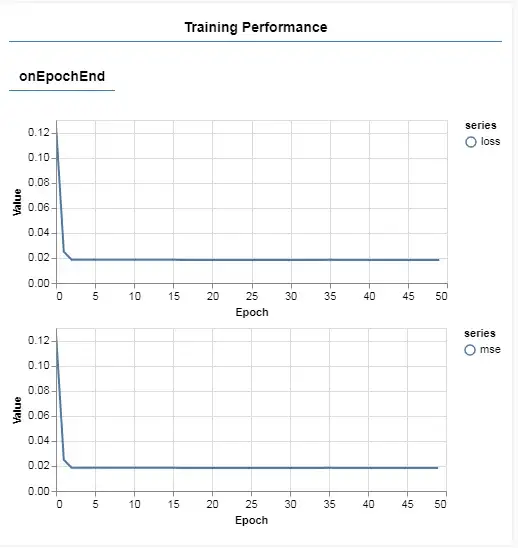
These are created by the callbacks we created earlier. They display the loss (on the most recent batch) and mse (on the whole dataset) at the end of each epoch.
When training a model we want to see the loss go down. In this case, because our metric is a measure of error, we want to see it go down as well.
Step 6: Make Predictions
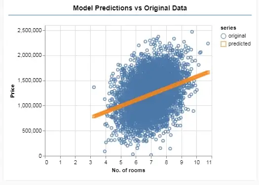
Now that our model is trained, we want to make some predictions. Let’s evaluate the model by seeing what it predicts for a uniform range of numbers of low to a high number of rooms.
Add the following function to your script.js file
function testModel(model, inputData, normalizationData) {
  const {inputMax, inputMin, labelMin, labelMax} = normalizationData;

  // Generate predictions for a uniform range of numbers between 0 and 1;
  // We un-normalize the data by doing the inverse of the min-max scaling
  // that we did earlier.
  const [xs, preds] = tf.tidy(() => {

    const xs = tf.linspace(0, 1, 100);
    const preds = model.predict(xs.reshape([100, 1]));

    const unNormXs = xs
      .mul(inputMax.sub(inputMin))
      .add(inputMin);

    const unNormPreds = preds
      .mul(labelMax.sub(labelMin))
      .add(labelMin);

    // Un-normalize the data
    return [unNormXs.dataSync(), unNormPreds.dataSync()];
  });


  const predictedPoints = Array.from(xs).map((val, i) => {
    return {x: val, y: preds[i]}
  });

  const originalPoints = inputData.map(d => ({
    x: d.rooms, y: d.price,
  }));


  tfvis.render.scatterplot(
    {name: 'Model Predictions vs Original Data'},
    {values: [originalPoints, predictedPoints], series: ['original', 'predicted']},
    {
      xLabel: 'No. of rooms',
      yLabel: 'Price',
      height: 300
    }
  );
}
A few things to notice in the function above.
const xs = tf.linspace(0, 1, 100);
const preds = model.predict(xs.reshape([100, 1]));
We generate 100 new ‘examples’ to feed to the model. Model.predict is how we feed those examples into the model. Note that they need to have a similar shape ([num_examples, num_features_per_example]) as when we did training.
// Un-normalize the data
const unNormXs = xs
  .mul(inputMax.sub(inputMin))
  .add(inputMin);

const unNormPreds = preds
  .mul(labelMax.sub(labelMin))
  .add(labelMin);
To get the data back to our original range (rather than 0–1) we use the values we calculated while normalizing, but just invert the operations.
return [unNormXs.dataSync(), unNormPreds.dataSync()];
.dataSync() is a method we can use to get a typedarray of the values stored in a tensor. This allows us to process those values in regular JavaScript. This is a synchronous version of the .data() method which is generally preferred.
Finally, we use tfjs-vis to plot the original data and the predictions from the model.
Add the following code to your run function.
testModel(model, data, tensorData);
Refresh the page and you should see something like the following once the model finishes training.
Congratulations! You have just trained a simple machine learning model using Tensorflow.js!


